Target pipeline
Note
If you are running the deprecated genericpipeline version of the pipeline (prefactor 3.2 or older), please check the old instructions page.
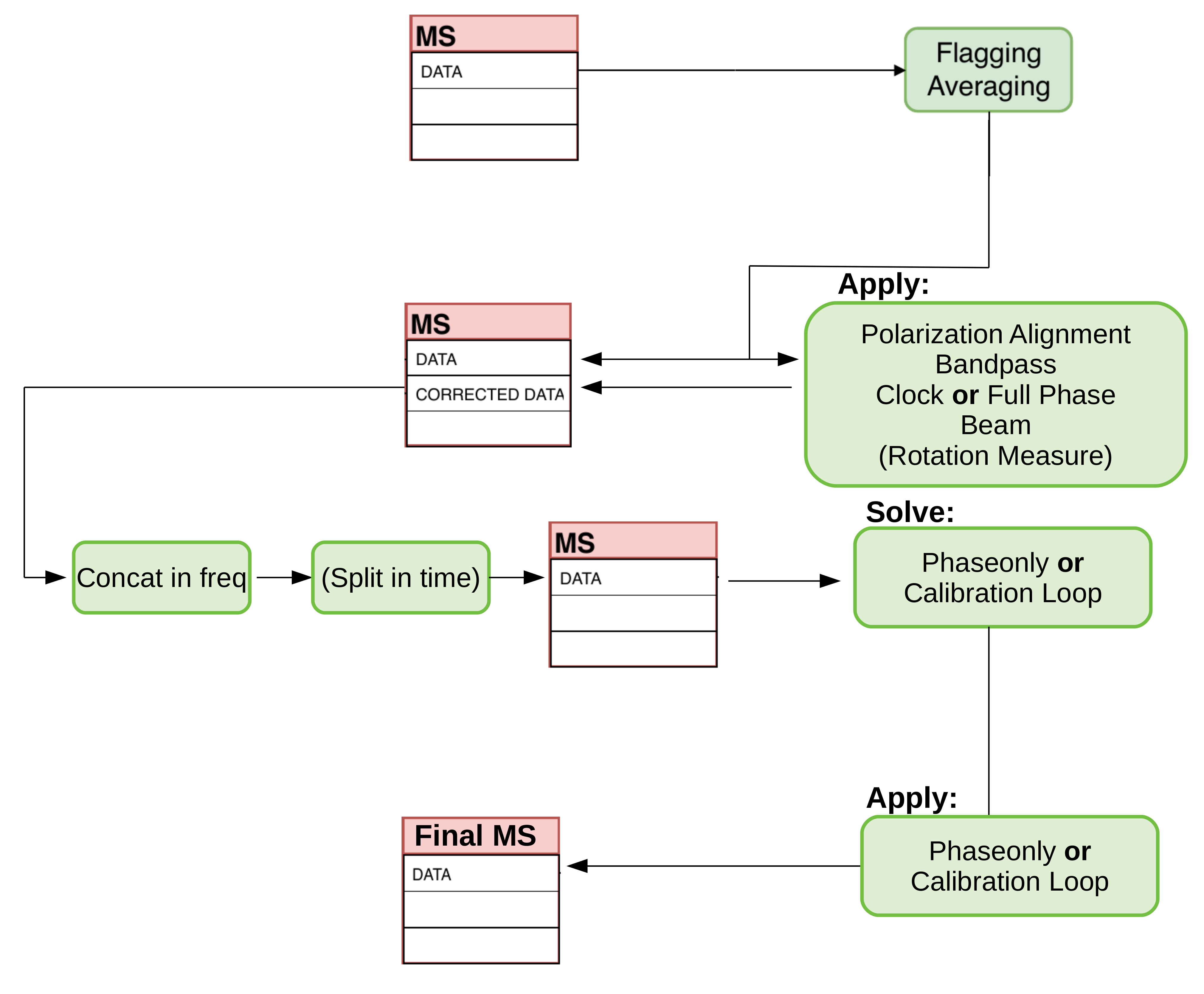
This pipeline processes the target data in order to apply the direction-independent corrections from the calibrator pipeline. A first initial direction-independent self-calibration of the target field is performed, using a global sky model based on the TGSS ADR or the new Global Sky Model (GSM), and applied to the data.
This chapter will present the specific steps of the target pipeline in more detail.
All results (diagnostic plots and calibration solutions) will be stored usually in the --outdir directory specified with your cwltool or toil command.
Prepare target, incl. “demixing” (prep)
This part of the pipeline prepares the target data in order to be calibration-ready for the first direction-independent phase-only self-calibration against a global sky model. This mainly includes mitigation of bad data (RFI, bad antennas, contaminations from A-Team sources), selection of the data to be calibrated (e.g. Dutch stations only), and some averaging to reduce data size and enhance the signal-to-noise ratio if applicable. Furthermore, for HBA observations ionospheric Rotation Measure corrections are applied, using spinifex The user can specify whether to do raw data or pre-processed data flagging. Demixing is performed only if the pointing is closer than 30 degress to an A-Team source if not specified by the user otherwise.
The basic workflows are:
preparation of data (
prep)concatenating and phase-only self-calibration against a global sky model (
gsmcal)creating the finally calibrated data set, via applying the self-calibration solutions and compressing the data (
finalize)
The workflow prep consists of:
- getting ionospheric Rotation Measure corrections and adding it to the solutions (step createRMh5parm)
retrieving and creating a global sky model containing A-Team sources (steps
find_skymodel_target,merge_skymodels)check for a potential station mismatch between calibrator solutions and the target data (step
compare_station_list)checking for nearby A-Team sources and determine which and how to demix them (step
check_Ateam_separationandcheck_demix).
Note
Demixing aims to remove the interference caused by strong outlier sources. The settings of various hyperparameters for demixing each particular observation are determined. The objective of fine-tuning various hyperparameters is to get the best removal of such outlier sources, whilst incurring minimal computational cost. In order to do this determination, all possible configurations of the hyperparameters are tested with a small sample of the observed data, and some information theoretic criteria are used for selecting the optimal configuration. On top of this, a set of pre-defined rules are also applied to this determination, much like human reasoning.
- basic flagging, applying solutions, and averaging (subworkflow
dp3_prep_target) edges of the band (
flagedge) – only used ifraw_data : truestatistical flagging (
aoflag) – only used inraw_data : truebaseline flagging (
flagbaseline)low elevation flagging (below 15 degress elevation) (
flagelev)low amplitude flagging (below 1e-30) (
flagamp)demix A-Team sources (
demix)applying calibrator solutions (steps
applyPA,applybandpass,applyclock,applyphase,applybeam,applyRM)averaging of the data in time and frequency
clipping time- and frequency chunks that are likely to be affected by A-Team sources and which have not been demixed before (step
clipper)
- basic flagging, applying solutions, and averaging (subworkflow
Calibration against a global skymodel (gsmcal)
These steps aim for deriving a good first guess for the phase correction in the direction of the phase center (direction-independent phase correction).
Once this is done, the data is ready for further processing with direction-dependent calibration techniques, using software like Rapthor, factor or killMS.
The phase solutions derived from the gsmcal workflow are collected and loaded into LoSoTo to provide diagnostic plots:
ph_freq??.png: matrix plot of the phase solutions with time for a particular chunk of target data, where both polarizations are colorcoded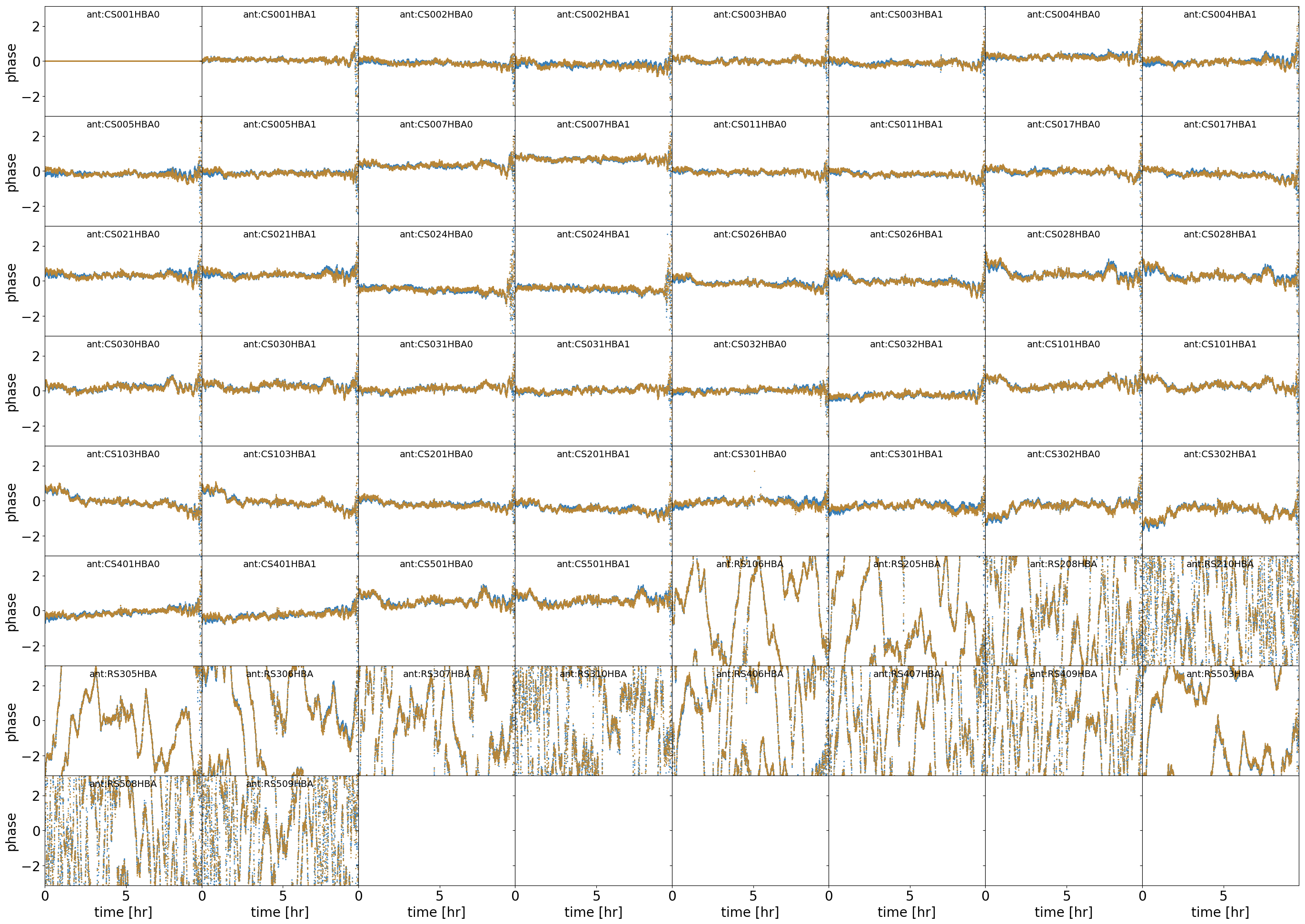
ph_poldif_freq??.png: matrix plot of the XX-YY phase solutions with time for a particular chunk of target data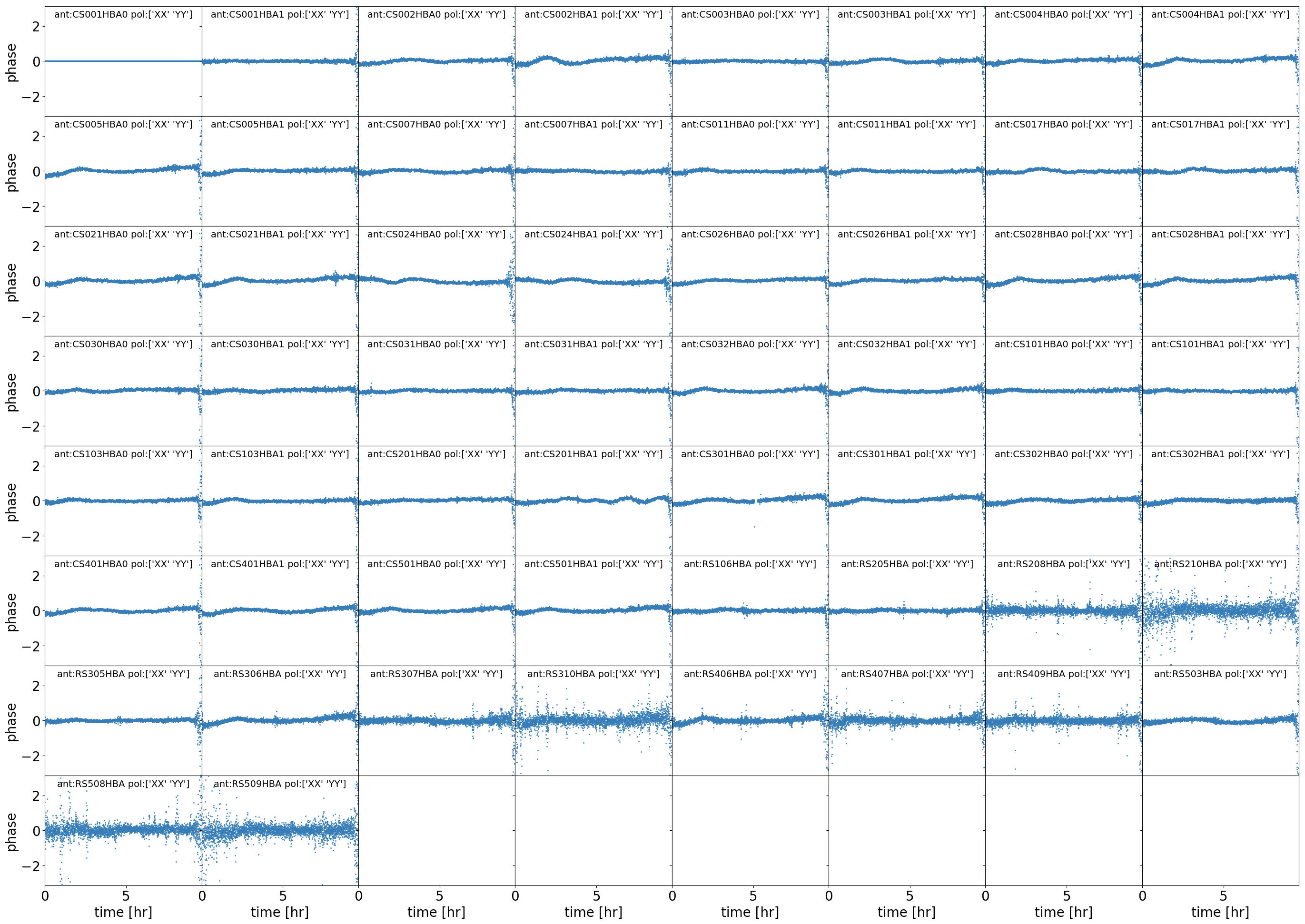
ph_pol??.png: matrix plot of the phase solutions for the XX and YY polarization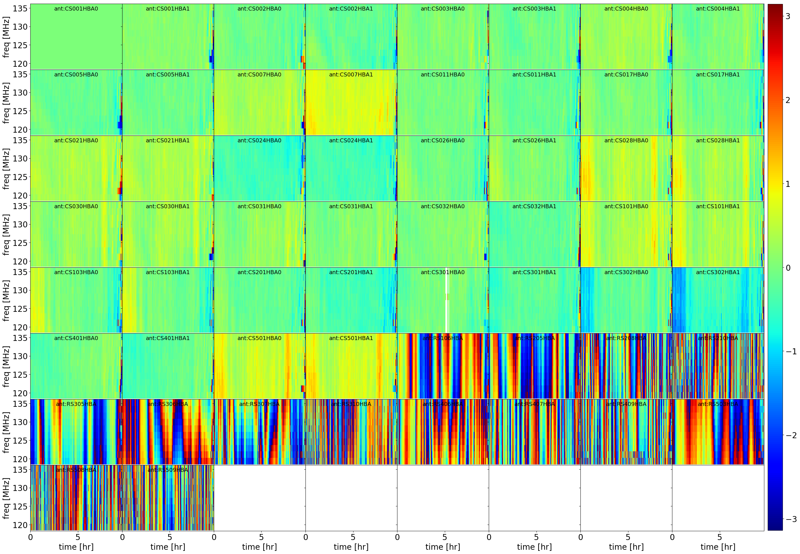
ph_poldif.png: matrix plot of the phase solutions for the XX-YY polarization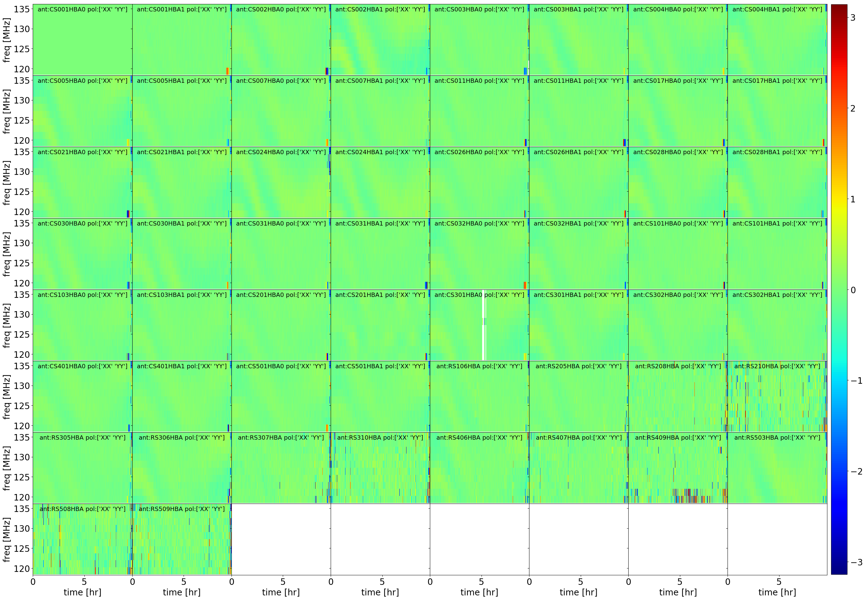
The plots always show the final solutions applied to the data. If run with selfcal: true, the solution plots for the calibration against the global skymodel are saved additionally for reference (e.g., ph_TGSS in case of skymodel_source: TGSS)
The workflow gsmcal consists of:
identification of fully flagged antennas (step
identify_bad_antennas)concatenating the data into chunks (subworkflow
concat)wide-band statistical flagging (steps
ms_concatandaoflag)checking for bad data chunks (step
check_unflagged_fraction)perform the calibration against the global skymodel using the full bandwidth (step
calibrate_target)perform self-calibration against a skymodel derived from imaging the dataset (subworkflow
selfcal_target_lbafor LBA observations andselfcal_target_hba(optional) for HBA observations)identifies bad core stations based on the phase solutions and removes them from the data (steps
losoto_flagstationandfind_flagged_antennas)
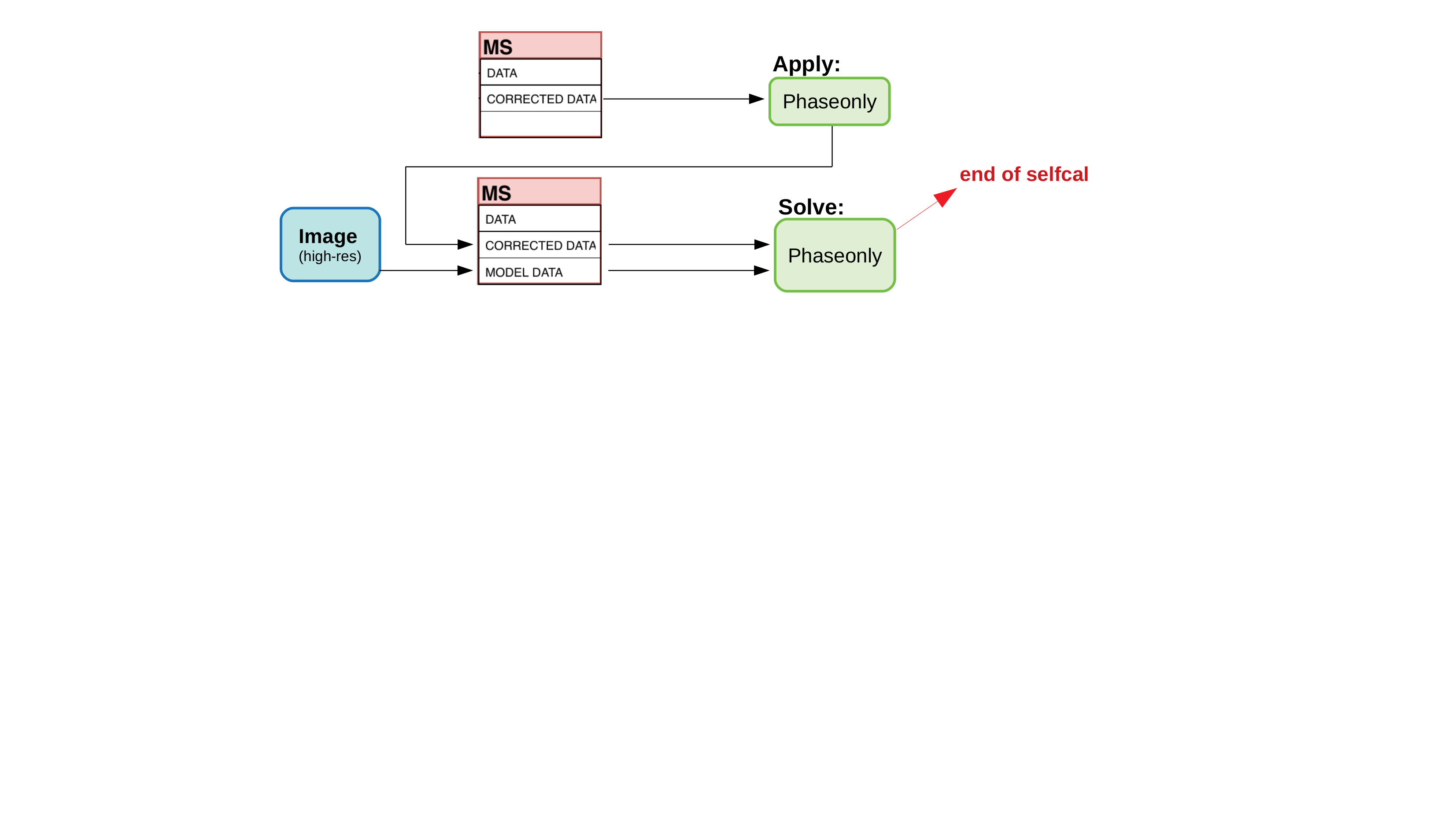
Self-calibration workflow for HBA observations (selfcal_target_hba)
The self-calibration procedure for LOFAR HBA observation is optional and highly recommended if the solutions derived from TGSS ADR or the new Global Sky Model (GSM) may have room for improvement.
??_??-MFS-image.fits: FITS image of the target field
- The workflow
selfcal_target_hbaconsists of: apply solutions derived from the calibration using TGSS ADR or the new Global Sky Model (GSM) (step
apply_gsmcal)image target field and write clean component model into model data column (step
image_target)perform the calibration against the model data column (subworkflow
self_calibrate_target, baseline-dependend smoothing (stepBLsmooth) if specifieddo_smooth : true)
Self-calibration workflow for LBA observations (selfcal_target_lba)
The self-calibration procedure for LOFAR LBA observations is run by default and aims for a more accurate determination of phase and amplitude corrections for the array than achieved using the Global Sky Model (GSM) only.
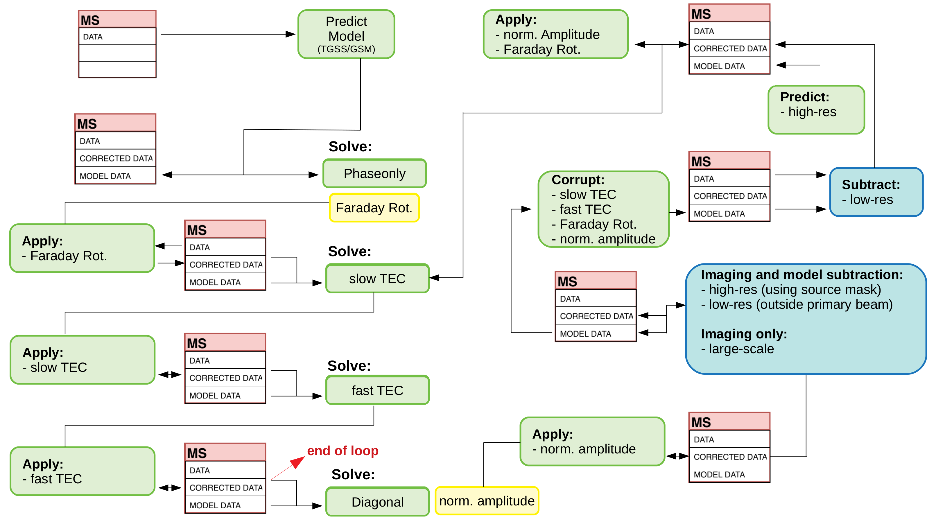
It requires an additional round of parameter extraction similar to the calibrator pipeline, starting from the correction of the effects caused by Faraday Rotation (workflow fr) as well as the Total Electron Content (TEC) and amplitude fluctuations (workflow tec_and_amp).
This is followed by imaging the calibrated data set at different resolutions to subtract the contamination from sources outside the primary beam of the telescope (workflow imaging_subtract) and update the skymodel in order to repeat the parameter extraction and correction (second iteration).
The final data set will have the sources outside the primary beam subtracted.
All solutions derived are loaded into LoSoTo to provide diagnostic plots:
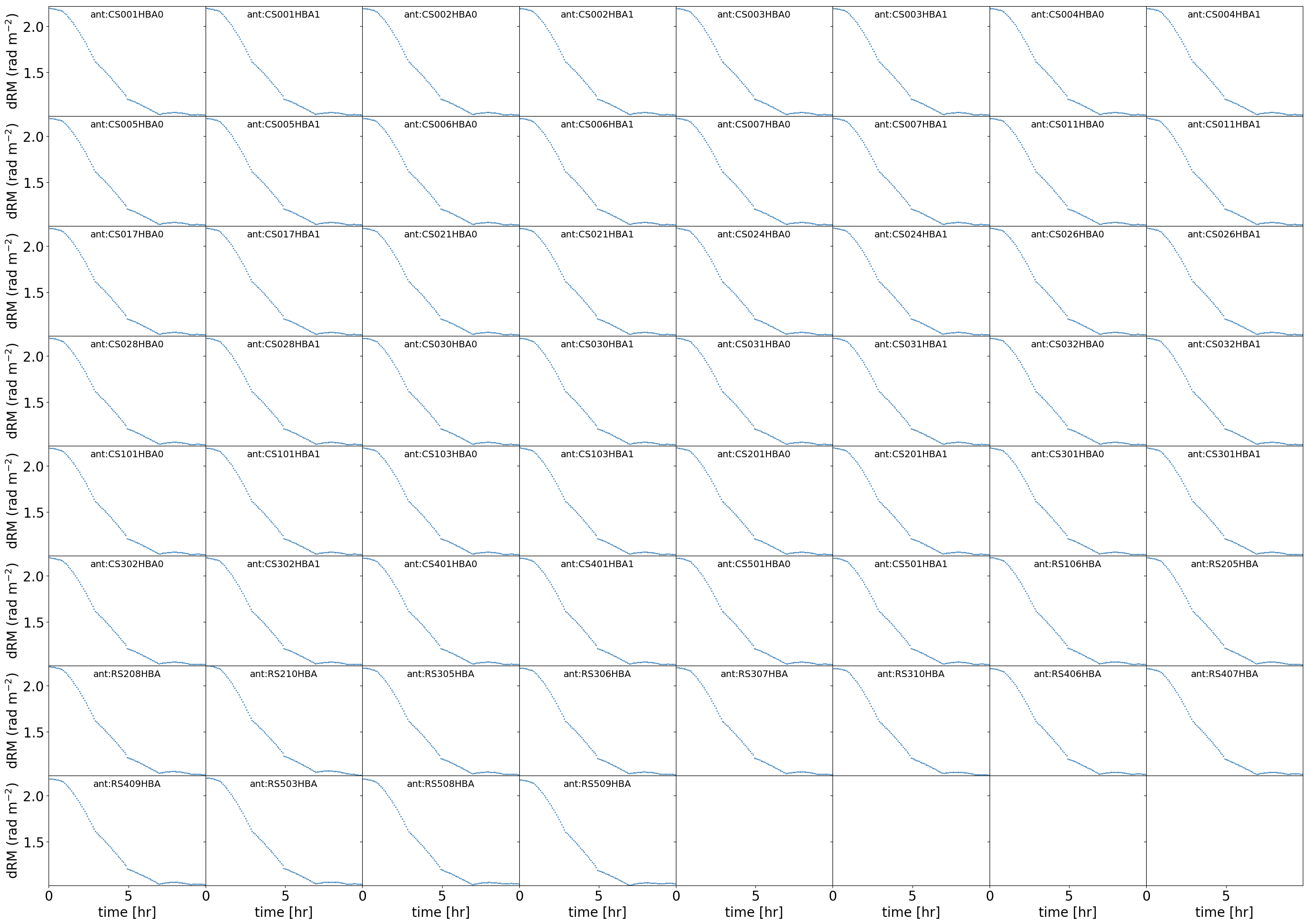
fr_ph_pol??.png: matrix plot of the phase solutions for the XX and YY polarizationfr_ph_poldif.png: matrix plot of the phase solutions from XX-YYfr: matrix plot of the derived differential Rotation Measure from Faraday Rotationslowtec?_freq??.png: matrix plot of the derived slow varying TEC values at a given calibration iteration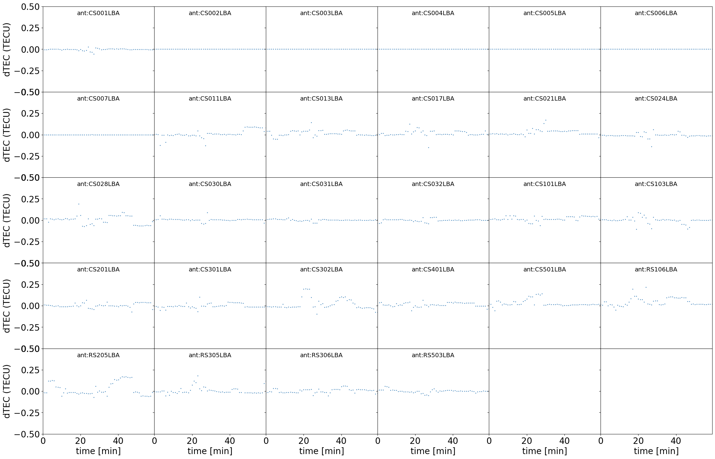
tec?_freq??.png: matrix plot of the derived fast varying TEC values at a given calibration iteration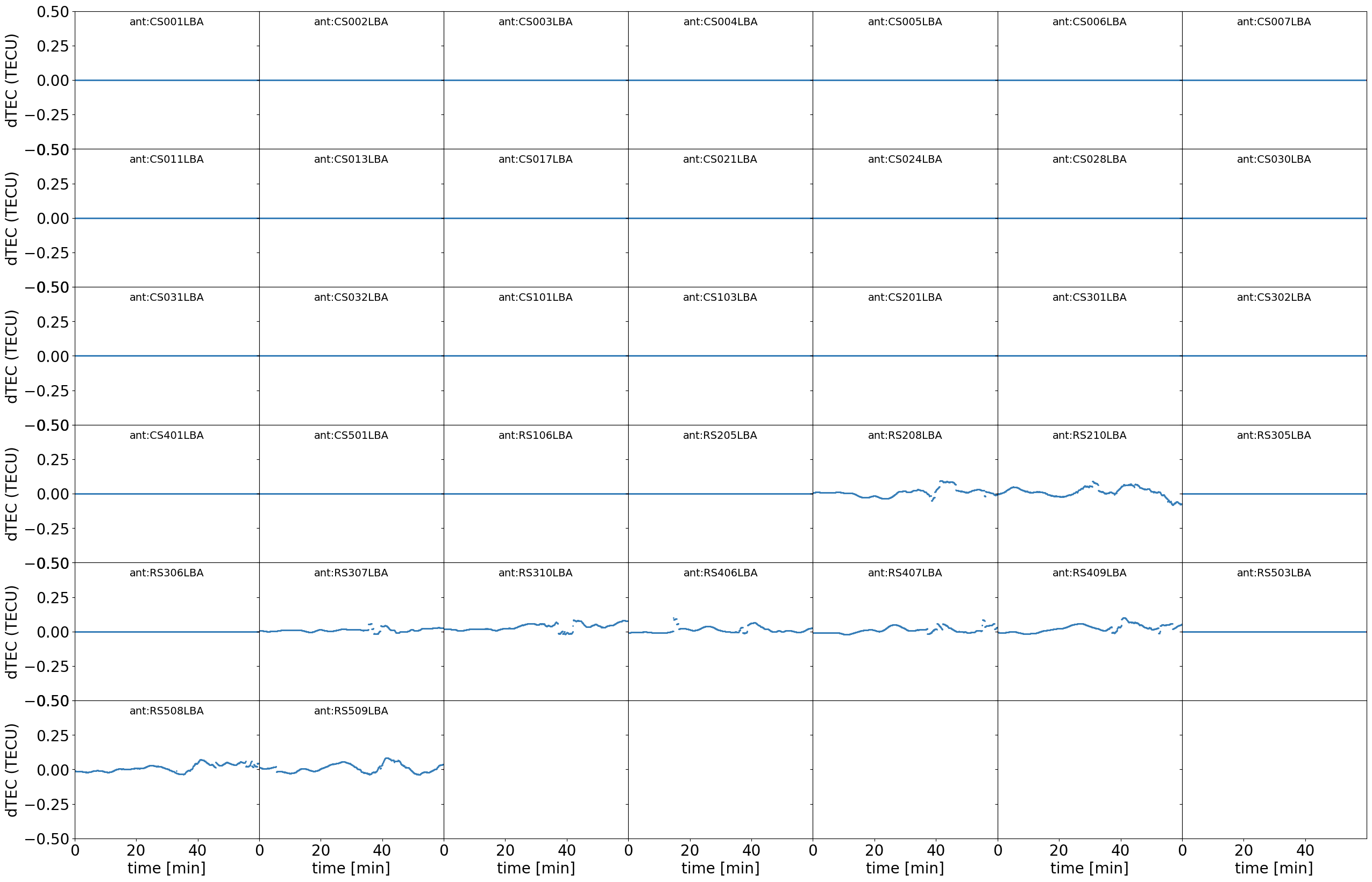
??_mask-MFS-image.fits: shallowly cleaned image at high resolution used as an input for determining a cleaning mask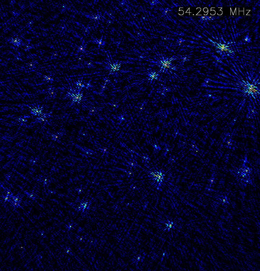
??.mask: derived cleaning mask from??_mask-MFS-image.fits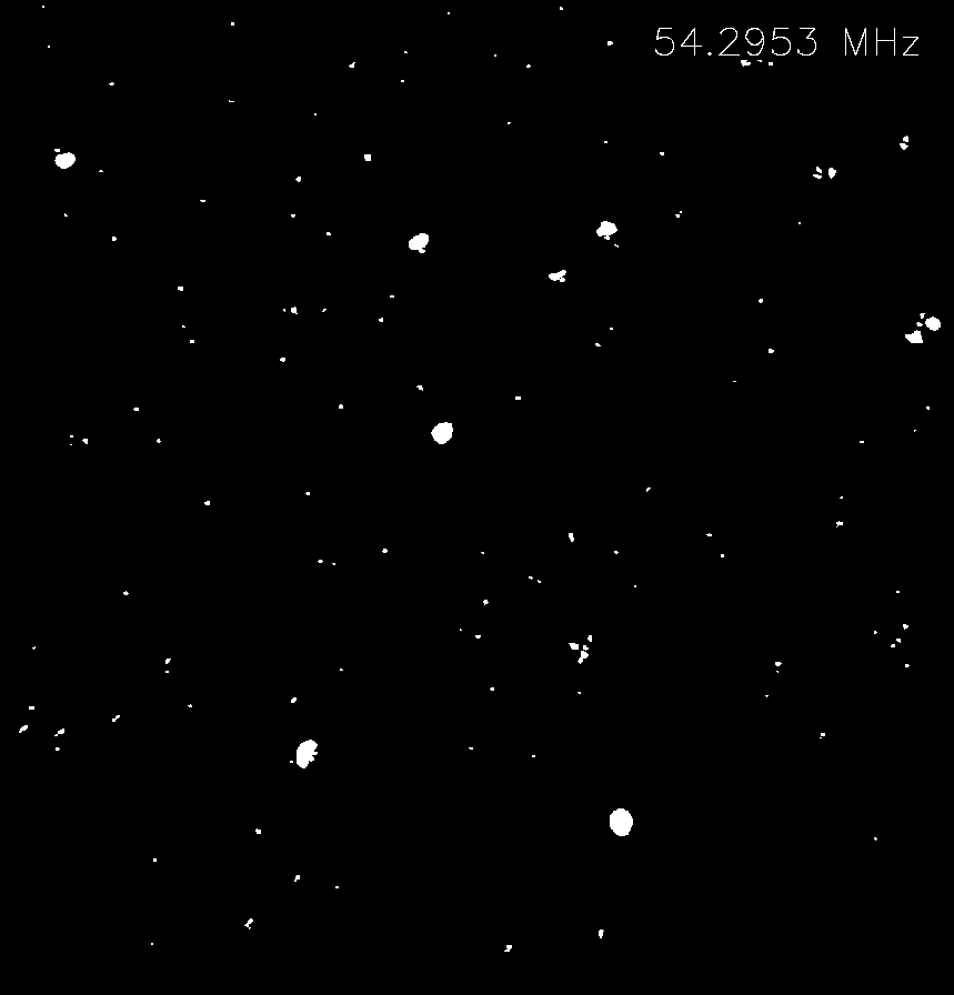
??_hires-MFS-image.fits: deeply cleaned high-resolution image using??.maskas a cleaning mask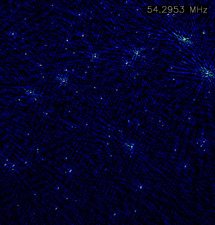
??_tmp-image.fits: shallowly cleaned image at low resolution after subtracting a model derived from the high-resolution image as a reference for the primary beam mask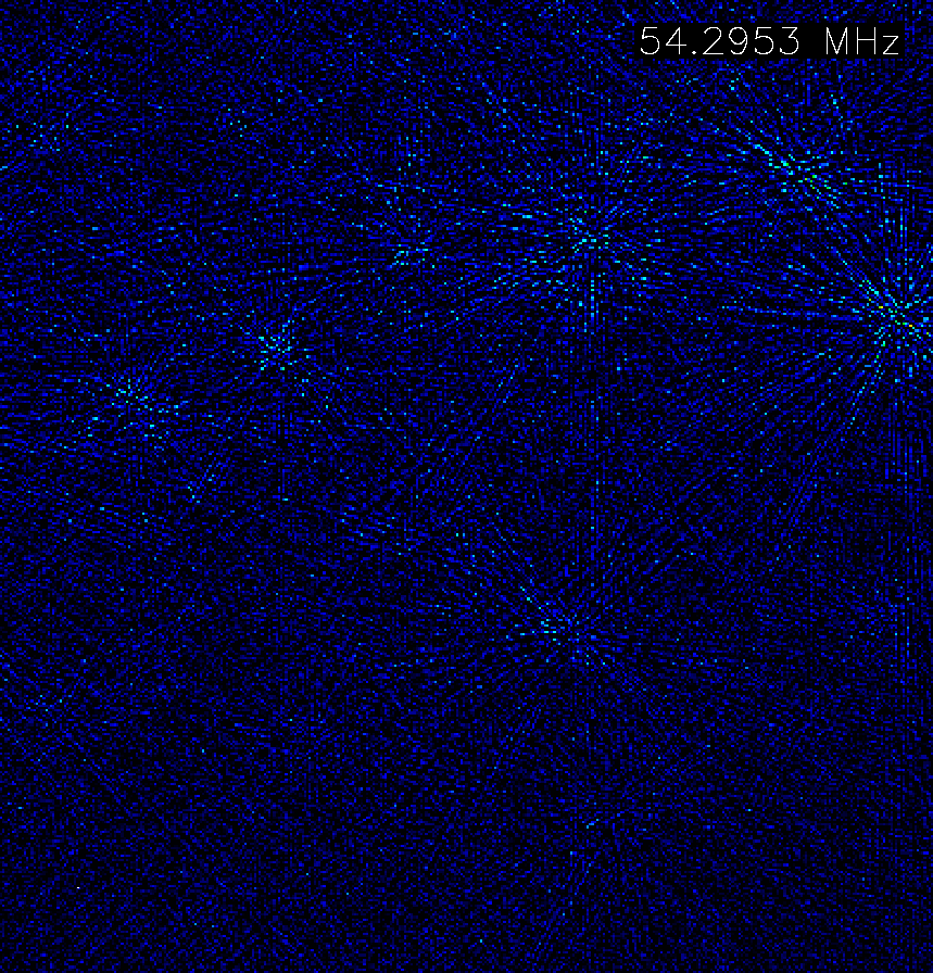
??_blank.fits: calculcated primary beam mask using??_tmp-image.fitsas a reference image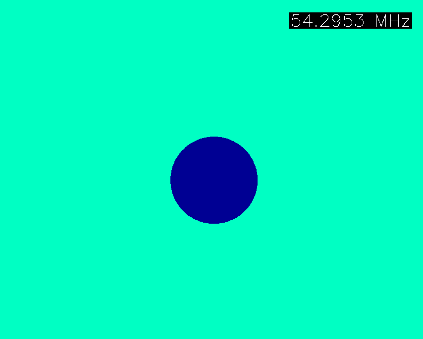
??_lowres-MFS-image.fits: deeply cleaned low-resolution image after subtracting a model derived from the high-resolution image using??_blank.fitsas a cleaning mask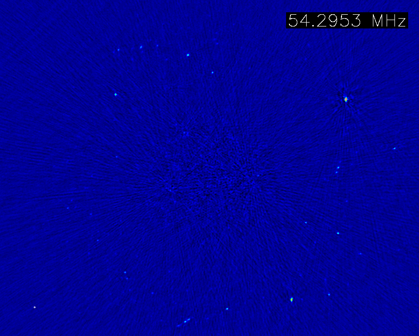
??_large-MFS-image.fits: diagnostic wide-field image at high resolution after subtracting a model derived from the low- and the high-resolution images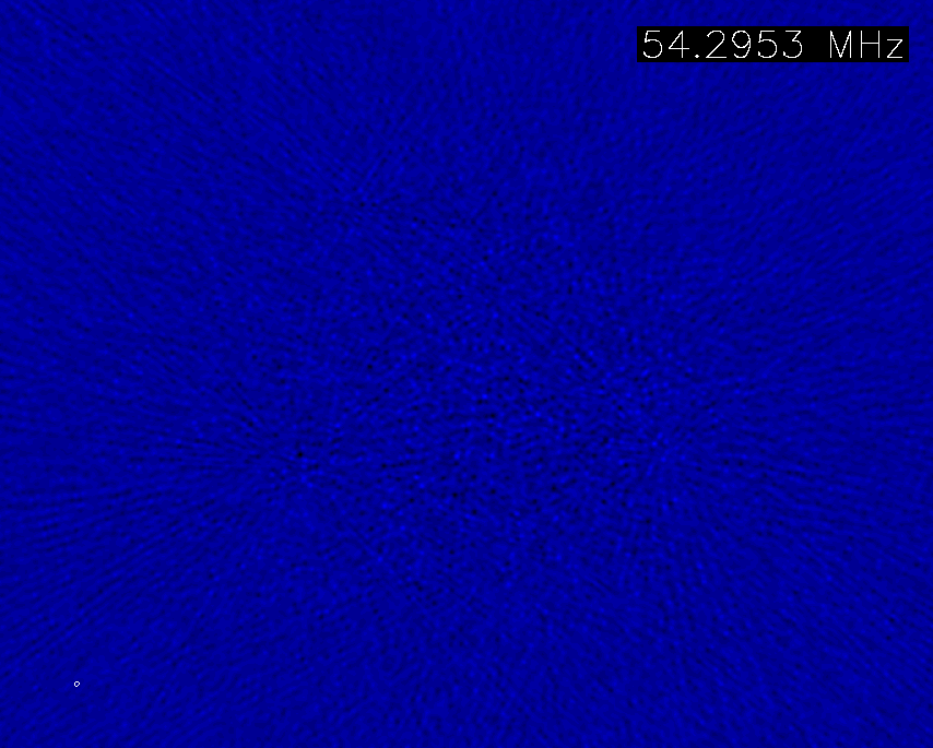
- The workflow
selfcal_target_lbaconsists of: create and calibrate against model data for Faraday Rotation (subworkflow
predict_calibrate_fr) and determination of the corresponding correction factors (subworkflowFaradayRot), create diagnostic plots (stepslosoto_plot) (subworkflowfr)apply corrections for Faraday Rotation correction and calibrate and correct for slow and fast varying ionospheric effects caused by the ionosphere as well as amplitude fluctuations (steps
apply_targ,calib_targ1,apply_targ1,calib_targ2, plus only in first loopapply_targ2,calib_targ_ampin subworkflowapply_calibrate_tec), create diagnostic plots (stepslosoto_plot) (subworkflowtec_and_amp, baseline-dependend smoothing (stepBLsmooth) is used.)correction of amplitude fluctuations (step
apply_targ_amp)imaging at high-resolution (step
image_hires) using an imaging mask (stepsmake_mask_image,make_mask), subtracting it from the data (stepspredict_hiresandsubtract_hires), imaging at low resolution (stepimage_lowres) outside the primary beam using an imaging mask (stepsimage_tmpandblank_image_reg), subtracting it from the data (stepspredict_lowres,subtract_lowres), flagging on the residual data (stepaoflag_residual), reconstruct data set for second calibration iteration through subtracting the low-resolution model comprising of sources outside the primary beam from the data (stepscorrupt_slowtec,corrupt_tec,corrupt_fr,corrupt_amp,subtract_modelfrom the subworkflowcorrupt_model), update the model data using the high-resolution image for the next calibration iteration (steprecreate_model) (subworkflowimaging_subtract)correction of amplitude fluctuations again (step
apply_targ_amp_2)second iteration of appyling corrections for Faraday Rotation and calibration of slow and fast varying ionospheric effects (subworkflow
tec_and_amp_2)
Finalizing the LINC output (finalize)
These steps produce the final data output and many helpful diagnostics.
- The workflow
finalizeconsists of: applying the final (from the global skymodel or from self-calibration) phaseonly or (in case of LBA) TEC self-calibration solutions to the data and compress them (step
apply_gsmcal_final)derive the structure function of the phases (step
structure_function)make a fast image of the target field (steps
averageandwsclean)create plots of the
uv-coverage of the final data set (stepuvplot)applies all solutions and flags of the pipeline to the original (high-resolution) data set and concats them in the same way (step
apply_and_concat_hires, ifoutput_fullres_datais set totrue)create a summary file (step
summary)
The last step also incorporates full Dysco compression to save disk space. The fully calibrated data is stored in the DATA column of the final data set.
Note
All solutions are written in the h5parm file format via the steps H5parm_collector and called during all the workflows.
The solutions are stored in the final calibrator solution set cal_solutions.h5.
Further diagnostics
- The output directory will contain all relevant outputs of the current LINC run, once the pipeline has finished:
fully calibrated datasets in
results, concatenated withnum_SBs_per_groupsubbands per MS file and averaged, if desired (see averaging options below). The DATA column of each MS contains the calibrated data (with the direction-independent solutions applied).logfiles in
logssummary file (JSON format) in
??_LINC_target_summary.jsoncalibration solutions in
cal_solutions.h5inspection plots in
inspectionused and created skymodels during the pipeline run in
skymodels
The following diagnostic help to assess the quality of the data reduction:
Ateam_separation.png: shows the distance and the elevation of A-Team sources with respect to the analyzed observation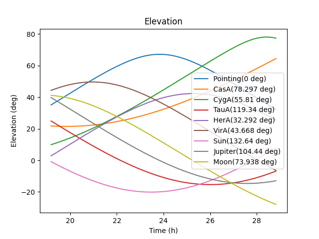
demix_solutions_??.png: shows the normalized amplitudes of the demixing solutions in time and frequency per station for the given direction
demix_noise_ratio.png: shows the reduction of the standard deviation noise after demixing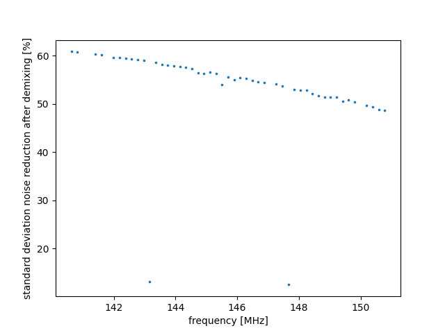
Ateamclipper.png: fraction of flagged data due to their potential contamination from A-Team sources versus frequency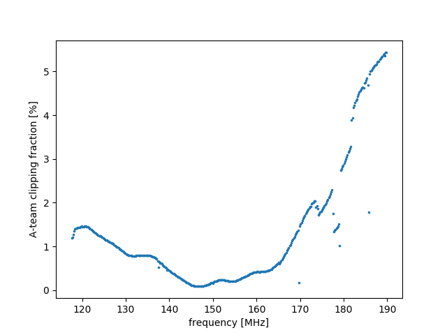
unflagged_fraction.png: fraction of remaining unflagged data versus frequency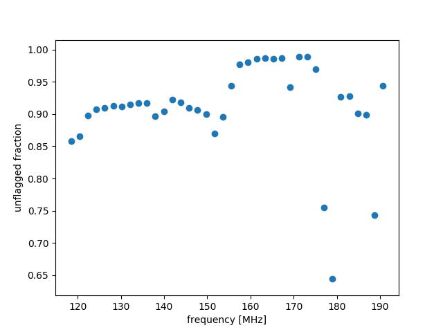
??_uv-coverage_uvdist.png: fraction of remaining unflagged data versusuv-distance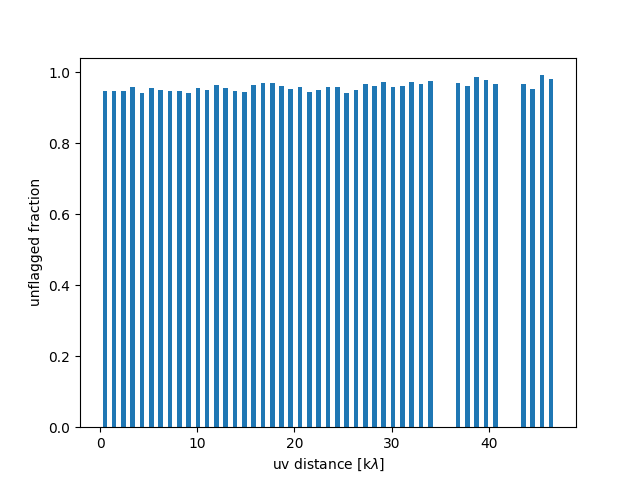
??_uv_coverage.png: theuv-coverage of the final data set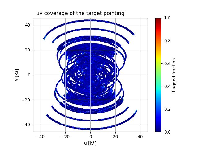
??_structure.png: plot of the ionospheric structure function of the processed target field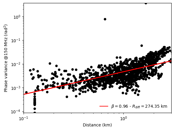
??-MFS-image.fits: FITS image of the target field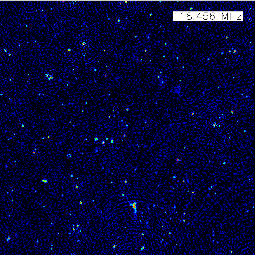
You can also check the calibration solutions for more details:
$ losoto -i cal_solutions.h5
Summary of cal_solutions.h5
Solution set 'calibrator':
==========================
Directions: 3c286
Stations: CS001HBA0 CS001HBA1 CS002HBA0 CS002HBA1
CS003HBA0 CS003HBA1 CS004HBA0 CS004HBA1
CS005HBA0 CS005HBA1 CS006HBA0 CS006HBA1
CS007HBA0 CS007HBA1 CS011HBA0 CS011HBA1
CS017HBA0 CS017HBA1 CS021HBA0 CS021HBA1
CS024HBA0 CS024HBA1 CS026HBA0 CS026HBA1
CS028HBA0 CS028HBA1 CS030HBA0 CS030HBA1
CS031HBA0 CS031HBA1 CS032HBA0 CS032HBA1
CS101HBA0 CS101HBA1 CS103HBA0 CS103HBA1
CS201HBA0 CS201HBA1 CS301HBA0 CS301HBA1
CS302HBA0 CS302HBA1 CS401HBA0 CS401HBA1
CS501HBA0 CS501HBA1 RS106HBA RS205HBA
RS208HBA RS210HBA RS305HBA RS306HBA
RS307HBA RS310HBA RS406HBA RS407HBA
RS409HBA RS503HBA RS508HBA RS509HBA
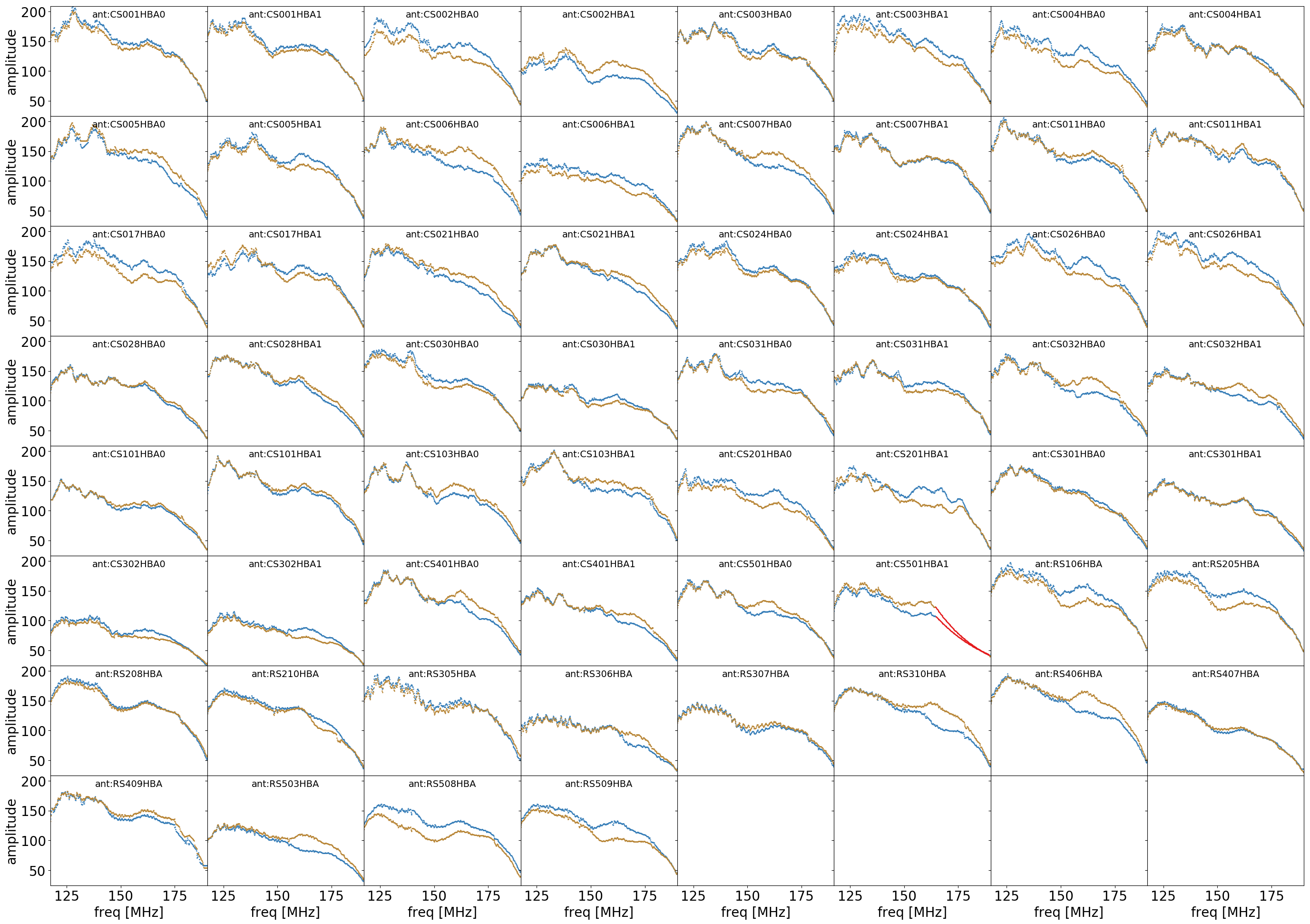
Solution table 'bandpass' (type: amplitude): 120 times, 372 freqs, 60 ants, 2 pols
Flagged data: 0.000%
Solution table 'clock' (type: clock): 120 times, 60 ants
Flagged data: 0.000%
Solution table 'faraday' (type: rotationmeasure): 60 ants, 120 times
Flagged data: 0.014%
Solution table 'polalign' (type: phase): 120 times, 60 ants, 1484 freqs, 2 pols
Flagged data: 0.000%
Solution set 'target':
======================
Directions: P000+00
Stations: CS001HBA0 CS001HBA1 CS002HBA0 CS002HBA1
CS003HBA0 CS003HBA1 CS004HBA0 CS004HBA1
CS005HBA0 CS005HBA1 CS006HBA0 CS006HBA1
CS007HBA0 CS007HBA1 CS011HBA0 CS011HBA1
CS017HBA0 CS017HBA1 CS021HBA0 CS021HBA1
CS024HBA0 CS024HBA1 CS026HBA0 CS026HBA1
CS028HBA0 CS028HBA1 CS030HBA0 CS030HBA1
CS031HBA0 CS031HBA1 CS032HBA0 CS032HBA1
CS101HBA0 CS101HBA1 CS103HBA0 CS103HBA1
CS201HBA0 CS201HBA1 CS301HBA0 CS301HBA1
CS302HBA0 CS302HBA1 CS401HBA0 CS401HBA1
CS501HBA0 CS501HBA1 RS106HBA RS205HBA
RS208HBA RS210HBA RS305HBA RS306HBA
RS307HBA RS310HBA RS406HBA RS407HBA
RS409HBA RS503HBA RS508HBA RS509HBA
Solution table 'spinifex' (type: rotationmeasure): 60 ants, 119 times
Flagged data: 0.000%
Solution table 'TGSSphase' (type: phase): 3446 times, 58 ants, 1 freq, 2 pols
Flagged data: 0.000%
History: 2021-07-30 11:25:44: Bad stations 'CS006HBA1', 'CS006HBA0' have not been added
back.
For an overall summary it is advised to check the summary logfile:
$ cat logs/???_summary.log

************************************
*** LINC target pipeline summary ***
************************************

Field name: P000+00

User-specified baseline filter: [CR]S*&
Additional antennas removed from the data: CS006HBA1, CS006HBA0
A-Team sources close to the phase reference center: NONE

XX diffractive scale: 4.4 km
YY diffractive scale: 4.0 km

Changes applied to cal_solutions.h5:
2021-07-30 11:25:44: Bad stations 'CS006HBA1', 'CS006HBA0' have not been added back.

Amount of flagged solutions per station and solution table:
Station   bandpass    clock    faraday  polalign  spinifex  TGSSphase
CS001HBA0    0.29%     0.00%     0.00%     0.00%     0.00%     0.00%
CS001HBA1    0.29%     0.00%     0.00%     0.00%     0.00%     0.00%
CS002HBA0    0.29%     0.00%     0.00%     0.00%     0.00%     0.05%
CS002HBA1    0.29%     0.00%     0.00%     0.00%     0.00%     0.00%
CS003HBA0    0.29%     0.00%     0.00%     0.00%     0.00%     0.00%
CS003HBA1    0.29%     0.00%     0.00%     0.00%     0.00%     0.05%
CS004HBA0    0.29%     0.00%     0.00%     0.00%     0.00%     0.05%
CS004HBA1    6.05%     0.00%     0.00%     0.00%     0.00%     0.05%
CS005HBA0    0.29%     0.00%     0.00%     0.00%     0.00%     0.05%
CS005HBA1    0.39%     0.00%     0.00%     0.00%     0.00%     0.00%
CS006HBA0    0.29%     0.00%     0.00%     0.00%     0.00%
CS006HBA1    0.29%     0.00%     0.00%     0.00%     0.00%

Amount of flagged data per station at a given state:
Station    initial  prep    Ateam   final
CS001HBA0   5.13%   5.41%  11.12%  22.74%
CS001HBA1   5.13%   5.41%  11.03%  22.51%
CS002HBA0   5.12%   5.39%  11.39%  23.18%
CS002HBA1   5.12%   5.40%  21.09%  29.95%
CS003HBA0   5.12%   5.39%   9.92%  22.58%
CS003HBA1   5.12%   5.40%  11.37%  23.95%
CS004HBA0   5.12%   5.40%  13.27%  24.62%
CS004HBA1   5.12%   5.40%  12.24%  23.53%
CS005HBA0   5.12%   5.40%  11.59%  23.38%
CS005HBA1   5.12%  15.36%  20.07%  30.09%
CS006HBA0 100.00% 100.00% 100.00%
CS006HBA1 100.00% 100.00% 100.00%

**********
Summary file is written to: ???_LINC_target_summary.json
Summary has been created.
User-defined parameter configuration
Parameters you will need to adjust
Location of the target data and calibrator solutions
msin: location of the input target data, for instructions look at the configuration instructions pagecal_solutions: location of the calibrator solutions, for instructions look at the configuration instructions page.
Parameters you may need to adjust
Data selection and calibration options
refant: regular expression of the stations that are allowed to be selected as a reference antenna by the pipeline (default:CS00.*)flag_baselines: DP3-compatible pattern for baselines or stations to be flagged (may be an empty list, i.e.:[])process_baselines_target: performs A-Team-clipping/demixing and direction-independent phase-only self-calibration only on these baselines. Choose[CR]S*&if you want to process only cross-correlations and remove international stations (default:[CR]S*&)filter_baselines: selects only this set of baselines to be processed. Choose[CR]S*&if you want to process only cross-correlations and remove international stations (default:[CR]S*&)do_smooth: enable or disable baseline-based smoothing (default:false)rfistrategy: strategy to be applied with the statistical flagger (AOFlagger, default:$LINC_DATA_ROOT/rfistrategies/lofar-hba-wideband.lua)min_unflagged_fraction: minimal fraction of unflagged data to be accepted for further processing of the data chunk (default:0.5)raw_data: use autoweight, set to True in case you are using raw data (default:false)compression_bitrate: defines the bitrate of Dysco compression of the data after the final step, choose 0 if you do NOT want to compress the datapropagatesolutions: use already derived solutions as initial guess for the upcoming time slothba_uvlambdamin: specify the minimum uv-distance in units of wavelength to be used when performing phase calibration with HBA (default:200)hba_uvmmax: specify the baselines with a maximum uv-distance in metre when performing phase calibration with HBA (default:1e15)maxStddev: maximum allowable standard deviation when outlier clipping is done. For phases, this value should be in radians, for amplitudes in log(amp). If None (or negative), a value of 0.1 rad is used for phases and 0.01 for amplitudes (default:-1.0)apply_tec: apply TEC solutions from the calibrator (default:false)apply_clock: apply clock solutions from the calibrator (default:true)apply_phase: apply full phase solutions from the calibrator (default:false)apply_RM: apply ionospheric Rotation Measure from spinifex (default:true)get_RM: downloads and extracts ionospheric Rotation Measure from spinifex (default:true). If set tofalse, the pipeline requires thetarget/spinifexsoltab to be already present in the input solutions provided bycal_solutionsifapply_RMis set totrue.apply_beam: apply element beam corrections (default:true)gsmcal_step: type of calibration to be performed in the self-calibration step (default:phase)updateweights: updateWEIGHT_SPECTRUMcolumn in a way consistent with the weights being inverse proportional to the autocorrelations (default:true)use_target: enable downloading of a target skymodel (default:true)skymodel_source: choose the target skymodel from TGSS ADR (TGSS), the Global Sky Model (GSM) or LoTSS-DR2 (LOTSS) (default:TGSS)skymodel_fluxlimit: limits the input skymodel to sources that exceed the given flux density limit in Jy (default:Nonefor HBA, i.e. all sources of the catalogue will be kept, and1.0for LBA)selfcal: perform self-calibration (default:false)selfcal_strategy: sets the strategy for selfcal. If set toHBA. If set toLBA, selfcal will perform extensive self-calibration according to the LiLF scheme (recommended for LBA observations). (default:HBA)selfcal_region: ds9-compatible region file to select the image regions used for the self-calibration in case of LBA self-calibration.selfcal_hba_imsize: specifies the image size in pixels, as a list, to use during HBA self-calibration (default:[20000, 20000]).calib_nchan: number of channels to be combined when performing phase (self-)calibration (default:1).output_fullres_data: additionally outputs full-resolution data sets concatenated according tonum_SBs_per_groupwith final phase solutions and flags applied (default:false)solveralgorithm: specifies the solver algorithm for the DP3 ddecal step (default:null, i.e. use the DP3 default).
A comprehensive explanation of the baseline selection syntax can be found here.
Skymodel directory
A-Team_skymodel: location of the A-Team skymodelstarget_skymodel: location of a user-defined target skymodel used for the self-calibration
Demixing and clipping options
demix: iftrueforce demixing using all sources ofdemix_sources, iffalsedo not demix at all, ifnullautomatically determines sources to be demixed according tomin_separation, considering the sources provided bydemix_sources(default:null)demix_sources: choose sources to be considered for demixing (provided as list, have to be a patch in the demix skymodel given byA-Team_skymodel), e.g.,[CasA,CygA](default:[VirA_Gaussian,CygA_Gaussian,CasA_Gaussian,TauA_Gaussian])demix_freqres: frequency resolution used when demixing (default:null, i.e. will be determined, typically 48.82kHz, which translates to 4 channels per subband, to be provided as string with units)demix_timeres: time resolution used when demixing in seconds (default:null, i.e. will be determined, typically 10)demix_maxiter: maximum amount of iterations to be used for demixing (default:null, i.e. will be determined, typically 20)lbfgs_historysize: for the LBFGS solver: the history size, specified as a multiple of the parameter vector, to use to approximate the inverse Hessian (default:null, i.e. will be determined, typically 10)lbfgs_robustdof: for the LBFGS solver: the degrees of freedom (DOF) given to the noise model (default:null, i.e. will be determined, typically 200)clipAteam: enables A-Team clipping using the source list fromclip_sources(default:true)clip_sources: list of the skymodel patches to be used for Ateamclipping, except those which are chosen to be demixed. An empty list means including all sources (enforced, not taking care whether demix is performed or not). (default:[VirA_Gaussian,CygA_Gaussian,CasA_Gaussian,TauA_Gaussian])min_separation: minimal accepted distance to an A-Team source on the sky in degrees. If the source is closer than that LINC will try to determine whether and how to demix (ifdemix: nulland will raise a WARNING, default:30)use_dnn: use the deep neural network model to determine demix parameters, if PyTorch is available (default:false)
Parameters for pipeline performance
max_dp3_threads: number of threads per process for DP3 (default:10)memoryperc: maximum of memory used for aoflagger in raw_flagging mode in percent (default:20)aoflag_reorder: make aoflagger reorder the measurement set before running the detection. This prevents that aoflagger will use its memory reading mode, which is faster but uses more memory (default:false, see the AOFlagger manual`_)aoflag_chunksize: this will split the set into intervals with the given maximum size, and flag each interval independently. This lowers the amount of memory required (default:2000)aoflag_freqconcat: concatenate all subbands on-the-fly before performing flagging. Disable if you use time-chunked input data (seechunkduration) (default:true)wsclean_tmpdir: Set the temporary directory ofwscleanused when reordering files (default:/tmp). CAUTION: This directory needs to be visible for LINC, in particular if you use Docker or Singularity.make_structure_plot: Calculate and plot the structure function of thegsmcal_step(only ifgsmcal_stepis set tophase, default:true)
Averaging for the target data
avg_timeresolution: intermediate time resolution of the data in seconds after averaging (default:4)avg_freqresolution: intermediate frequency resolution of the data after averaging (default:48.82kHz, which translates to 4 channels per subband)avg_timeresolution_concat: final time resolution of the data in seconds after averaging and concatenation and before phase calibration (default:8)avg_freqresolution_concat: final frequency resolution of the data after averaging and concatenation and before phase calibration (default:97.64kHz, which translates to 2 channels per subband)
Concatenating of the target data
num_SBs_per_group: make concatenated measurement-sets with that many subbands (default:10)reference_stationSB: station-subband number to use as reference for grouping (default:None-> use lowest frequency input data as reference)chunkduration: Duration (in seconds) after which to start writing a next measurement set while concatenating (default: 0.0, no chunking in time)