Image pipeline

This pipeline produces a Stokes-I image (a Stokes-V image is also produced for quality-control purposes) of the full FOV of the target data, using the full bandwidth. The parset is named Pre-Facet-Image.parset.

Prepare target

The target data that result from the target pipeline are averaged and concatenated in preparation for imaging. The steps are as follows:

create_ms_map

Generate a mapfile of all the target data.

combine_mapfile

Generate a mapfile with all files in a single entry. This mapfile is used as input to the next step.

do_magic

Compute image sizes and the number of channels to use during imaging from the MS files from the previous step. The image size is calculated from the FWHM of the primary beam at the lowest frequency at the mean elevation of the observation. The number of channels is set simply as the number of subbands / 40, to result in enough channels to allow multi-frequency synthesis (MFS), but not so many that performance is impacted. A minimum of 2 channels is used.

do_magic_maps

Convert the output of do_magic into usable mapfiles.

average

Average the data as appropriate for imaging of the FOV. The amount of averaging depends on the size of the image (to limit bandwidth and time smearing). The averaging currently adopted is 16 s per time slot and 0.2 MHz per channel. These values result in low levels of bandwidth and time smearing for the target image sizes and resolutions.

combine_mapfile_deep

Generate a mapfile with all files in a single entry. This mapfile is used as input to the next step.

dpppconcat

Run DPPP to concatenate the data. Concatenating the data speeds up gridding and degridding with IDG by factors of several.

Imaging

WSClean is used to produce the Stokes-I/V images. See the parset and the do_magic step above for details of the parameters used. The values are chosen to produce good results for most standard observations.

wsclean_high_deep

Image the data with WSClean+IDG. Imaging is done in MFS mode, resulting in a single image for the full bandwidth. Primary-beam corrected and uncorrected images are made.

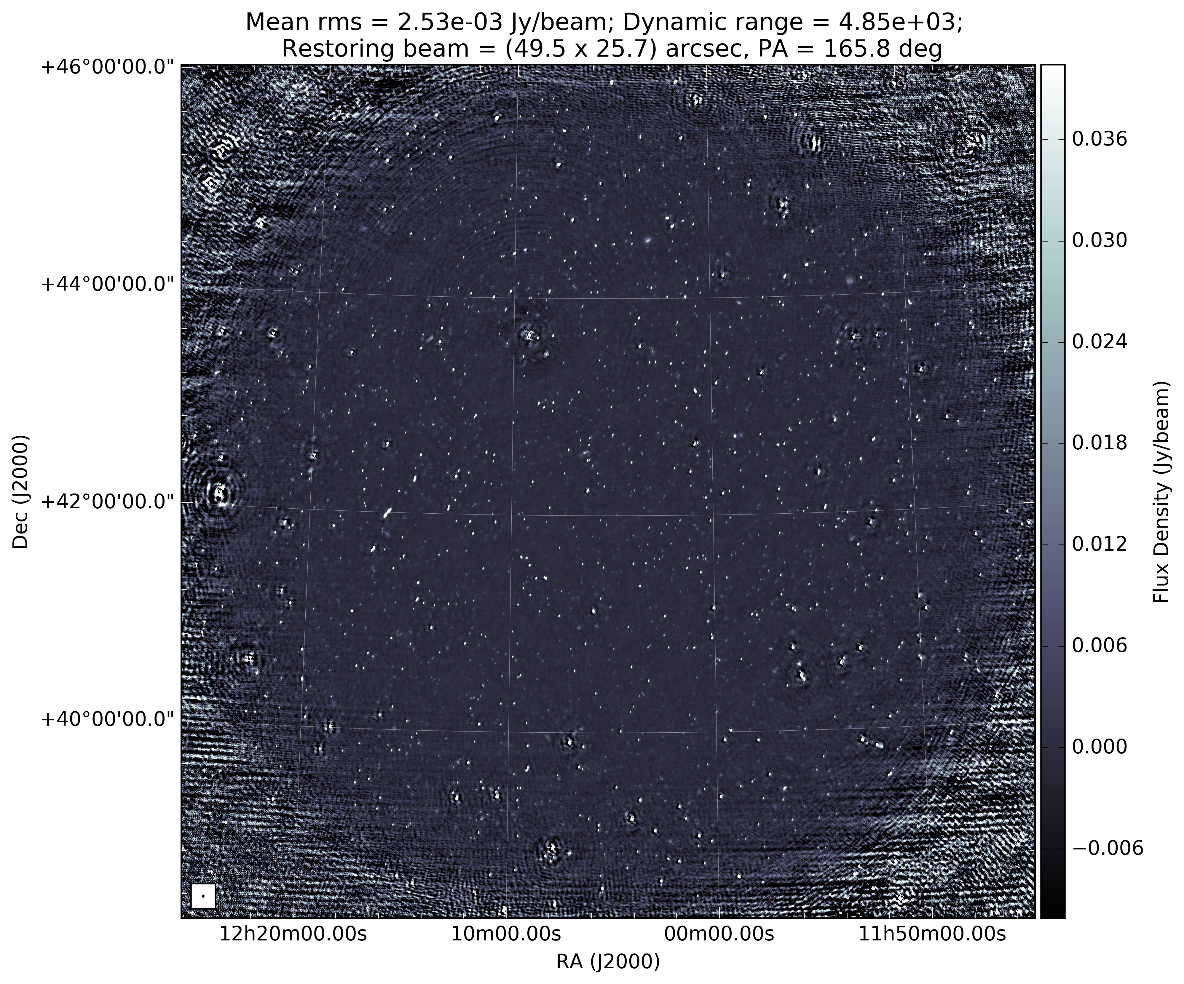
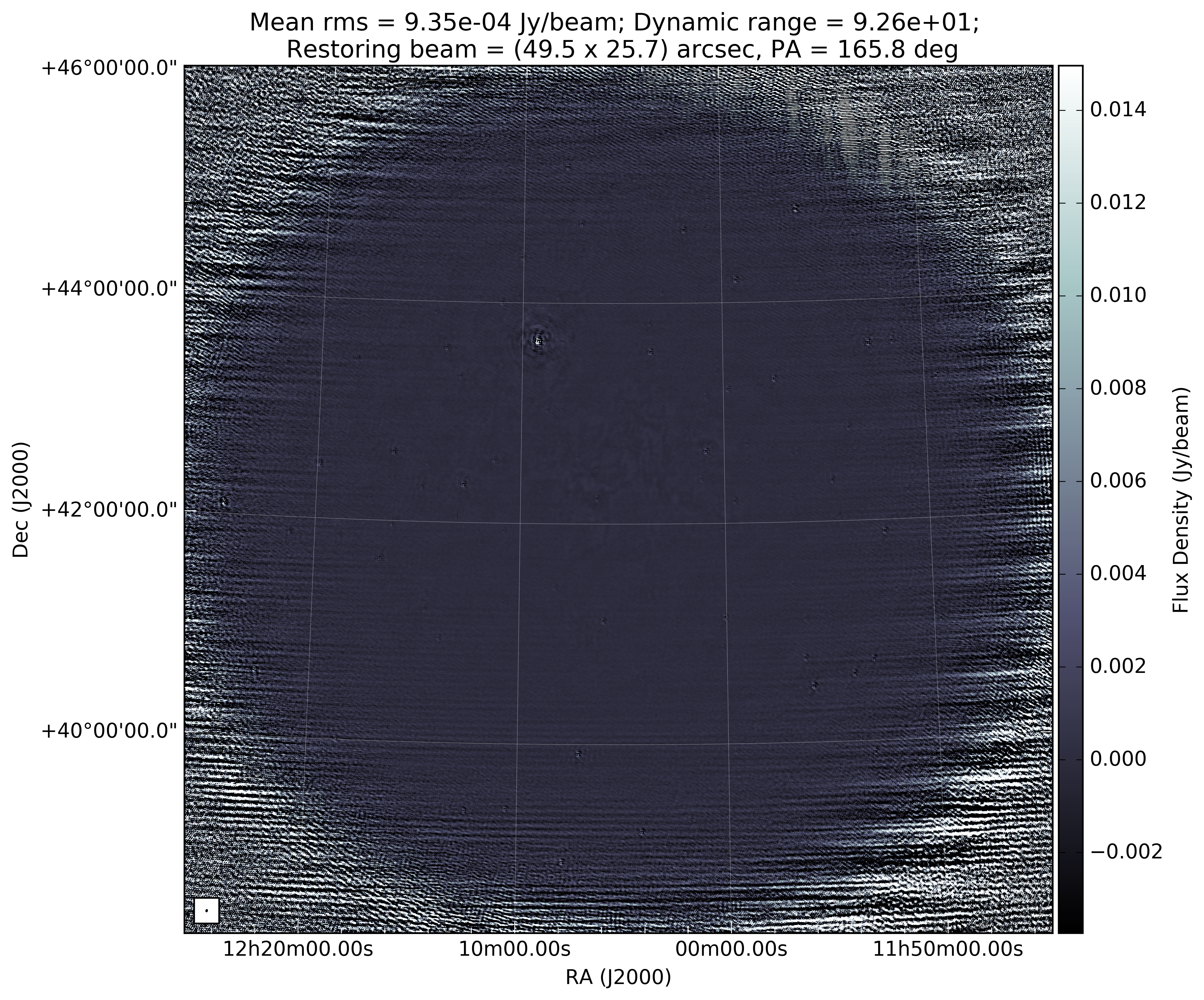
plot_im_high_i/v

Make a png figure of the Stokes-I/V images, including estimates of the image rms and dynamic range and the restoring beam size. Typical HBA images look like the ones below (Stokes-I image is shown first and the Stokes-V image second).

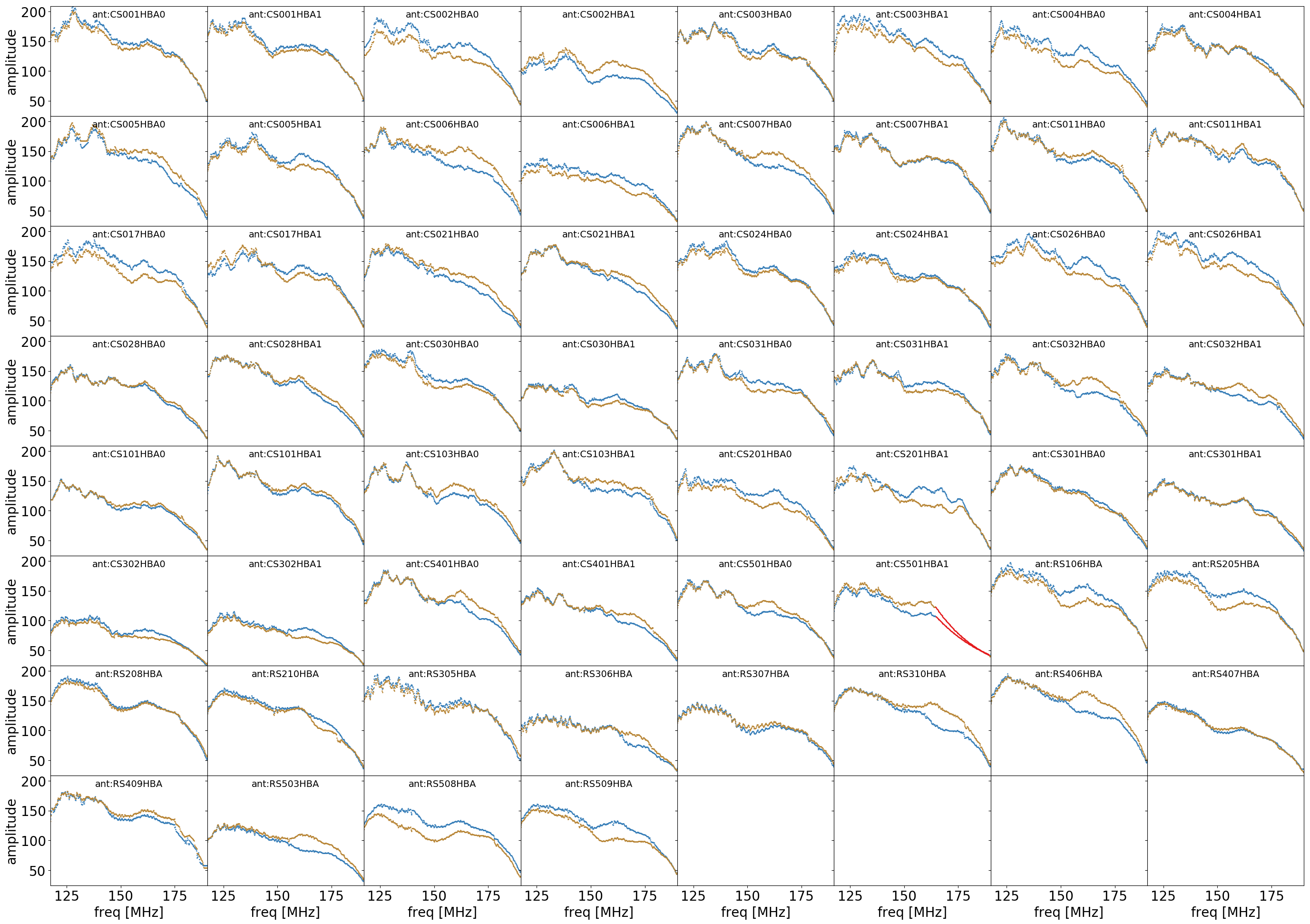
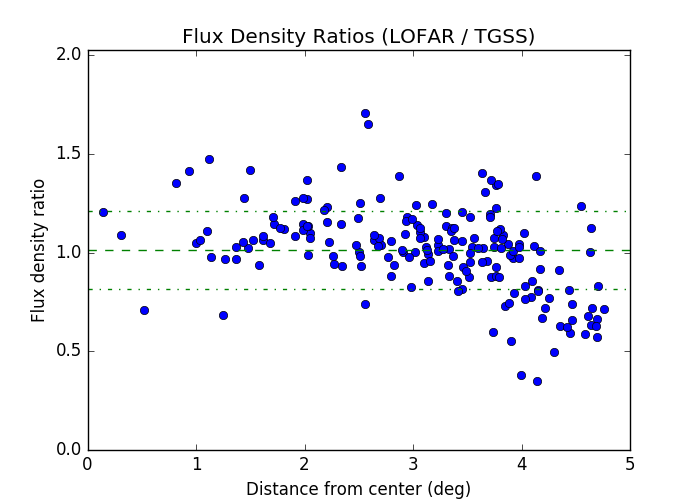
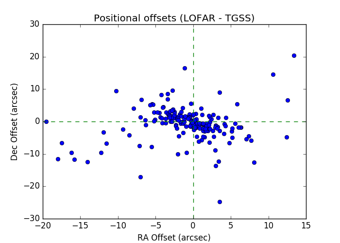
make_source_list

Make a list of sources from the Stokes-I image using PyBDSF and compare their properties to those of the TGSS and GSM catalogs for HBA and LBA data, respectively. A number of plots are made to allow quick assessment of the flux scale and astrometry of the image:

User-defined parameter configuration

Information about the input data

! target_input_path

Directory where your concatenated target data are stored.

! target_input_pattern

Regular expression pattern of all your target files.

Note

These files should have the direction-independent calibration applied to the DATA column (usually the *.pre-cal.ms files from the target pipeline).

Imaging parameters

• cellsize_highres_deg

  Cellsize in degrees (default: 0.00208).

• fieldsize_highres

  Size of the image is this value times the FWHM of mean semi-major axis of the station beam at the lowest observed frequency (default: 1.5).

• maxlambda_highres

  Maximum uv-distance in lambda that will be used for imaging. A minimum uv-distance of 80 lambda is used in all cases (default: 7000).

• image_padding

  Amount of padding to add during the imaging (default: 1.4).

• idg_mode

  IDG mode to use: cpu or hybrid (default: cpu).

• local_scratch_dir

  Scratch directory for WSClean (default: {{ job_directory }}).

• image_rootname

  Output image root name (default: {{ job_directory }}/fullband). The image will be named image_rootname-MFS-I-image.fits.

Parameters for HBA and LBA observations

parameter	HBA	LBA
cellsize_highres_deg	0.00208	0.00324
maxlambda_highres	7000	4000